We left off the last post looping over each pixel, wahoo! So this final post will focus on ✨filter types✨.

Here’s the image I’m working against:

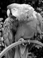
And here’s the final output of this post.

In the last post, we were splitting the scanline into individual rows and looping over each byte in the row. Conveniently enough, the sample image has a 1:1 pixel to byte ratio, so we don’t need to do anything special to group bytes together to make a more complex pixel, or split them up. But keep in mind that won’t always be the case.

You might’ve noticed in the last method we worked on, if a row was 150 pixels wide, we were always adding one additional byte to the row. That first byte of the row was added to a variable called filterByte. (You can refresh your memory here.)

So what is a filter byte? The concept is so clever! Let’s circle back to the baby blue rbg value I referenced in the last post: 137, 207, 240.

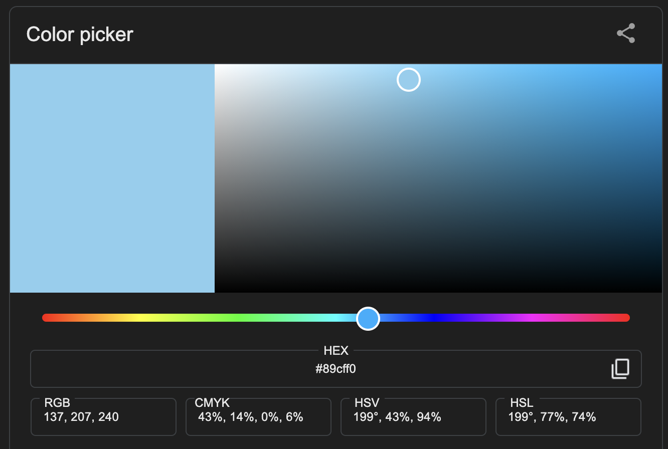
Converted to a byte array, that single pixel looks like this:

[ 10001001, 11001111, 11110000 ]

Of course, this is just a single pixel, think about an entire image. We already talked about how unwieldy this could get, but consider how often a single color gets repeated in an image. Look at the sample grayscale image we’re using - there’s a lot of the same colors. Think about how much space a file could save if it could use one complete pixel value as a reference for other pixels - that is what Filter Types do. 🤯

There are 5 different values for a filter type:

• 0: No filter is applied. The values for this row are absolute values
• 1: Sub filtering - performs a look behind to the pixel directly to its left
• 2: Up filtering - performs a “look up” to the pixel directly above it
• 3: Average filtering - takes an average of the neighboring pixels
• 4: Paeth filtering - using neighboring pixels, Paeth is predictive in choosing the value closest to the computed value

Let’s go through these one at a time. In the previous post, we left off looping over the row, but now let’s assume we’re passing the entire row to a function where the looping is performed.

// note that this function will assume that currentRow DOES NOT include filterByte
+ function applyPixelFilter(filterType, bitDepth, currentRow, previousRow) {
+   switch(filterType) {
+     case 0: 
+     case 1:
+     case 2:
+     case 3:
+     case 4:
+   }
+ }

Since a filter type of 0 means the pixels are already in their absolute form, we’ll start with filter type 1. As mentioned above, filter type 1 is performing a look-behind to it’s left-hand neighbor. The first row in a PNG might use this filter type, since it doesn’t have any neighbors above it for reference.

When the look-behind is performed, the current pixel doesn’t just assume the value of the previous pixel - instead the value is the combined total of the left-hand pixel and the current pixel, up to 255. Note that this number wraps around, so any overflow beyond 255 is the actual value used.

  /* ... */

  switch(filterType) {
    /* ... */

    case 1:
+   let unfilteredPixels = []

+   currentRow.forEach((value, i) => {
+     if (i === 0) {
+       unfilteredPixels.push(value)
+       return
+     }

      // perform look-behind
+     unfilteredPixels.push(
+       (value + (unfilteredPixels[unfilteredPixels.length - 1] || 0)) % 256
+     )
+   })

+   return unfilteredPixels

    /* ... */
  }

In our first case (as we will in every case) we loop over the row. (Note that you need to check for the bitDepth to make sure that a pixel really is a single byte, as this assumes. I left that out to keep the code more approachable.)

Within the loop, we are assuming that the first byte value is an absolute value, which is safe for a look-behind, because that pixel has no left-hand neighbor to reference. Moving on, we are using the last value from our unfilteredPixels array as our reference. It’s important to note that as we are looping over the row, each previous pixel was also referencing its left-hand neighbor. In order to calculate the correct value for the current pixel, we need to look at the absolute value of the previous pixel, which we receive after filtering, not the provided value. This will be true for all filter types.

Filter type 2 is very similar, but instead of a look-behind, it performs a “look-up”. Using previousRow as our reference, we will combine the current pixel’s value and the absolute value from the same space in the previous row.

  /* ... */

  switch(filterType) {
    /* ... */

    case 2:
+     let unfilteredPixels = []

+     currentRow.forEach((value, i) => {
        const b = previousRow?.[i] || 0

+       unfilteredPixels.push((value + b) % 256)
+     })

+     return unfilteredPixels

    /* ... */
  }

Filter type 3 is a little bit more complicated, but it builds on types 1 and 2. Instead of adding the absolute value of a neighboring pixel, we take the average of two neighboring pixels - left and above - and add their average to the current pixel’s value.

  /* ... */

  switch(filterType) {
    /* ... */

    case 3:
+   let unfilteredPixels = []

+   currentRow.forEach((value, i) => {
+     if (i === 0) {
+       const b = previousRow[i] || 0
+       const avg = Math.floor(b / 2)

+       unfilteredPixels.push((value + avg) % 256)

+       return
+     }

+     const a = unfilteredPixels[unfilteredPixels.length - 1] || 0
+     const b = previousRow[i] || 0

+     const avg = Math.floor((a + b) / 2)

+     unfilteredPixels.push((value + avg) % 256)
+   })

+   return unfilteredPixels

    /* ... */
  }

Similar to case 1, we know that the first pixel in this row will not have a left-hand neighbor, so we take the average of the neighborhood above, and add that value to the current pixel. Remember that we are always taking absolute values after the filtering has been applied.

Moving on in the loop, we take each reference value, and find their average. That average is then applied to the current pixel’s value.

Lastly, we have Paeth filtering, which is the most complicated. It uses three reference pixels: left, top, and top-left. It might look like this, where D is the current pixel:

C  B
A  D

Let’s look at a Paeth function in isolation:

// paeth takes in each of our reference values
function paeth(a, b, c) {
  // first find P -- that is your comparison
  const p = a + b - c

  // now that we have p as a comparison, we can find which initial value is closest to p
  // take the absolute value of the difference between p and the current value
  // compare that difference to the previous difference
  // if the new difference is lesser -- use it
  const leastDiffObj = [a, b, c].reduce(
    (prev, curr) => {
      const difference = Math.abs(p - curr)

      if (prev.difference === null) {
        return {
          value: curr,
          difference,
        }
      }

      const diffObj =
        difference < prev.difference ? { value: curr, difference } : prev

      return diffObj
    },
    {
      value: a,
      difference: null,
    }
  )

  return leastDiffObj.value
}

We use p as a comparision value for the rest of the reference values. p takes on the value of a+b-c. We loop over a, b, and c to find the value that is furthest from p, but note that we want the outcome to be less than p. So given p=30, a=20, b=20, and c=65, even though c is furthest from p, a would still win because it is a lesser value.

Now that we’ve completed the paeth function, we can apply its result.

  /* ... */

  switch(filterType) {
    /* ... */

    case 4:
+   let unfilteredPixels = []

+   currentRow.forEach((value, i) => {
+     if (i === 0) {
+       const b = previousRow[i]

+       unfilteredPixels.push((value + b) % 256)

+       return
+     }

+     const a = unfilteredPixels[unfilteredPixels.length - 1] || 0
+     const b = previousRow[i] || 0
+     const c = previousRow[i - 1] || 0

+     let difference = paeth(a, b, c)

+     unfilteredPixels.push((value + difference) % 256)
+   })

+   return unfilteredPixels

    /* ... */
  }

Similar to cases 1 and 3, if we are on the first index of a row, that index has neither a left-hand neighbor, or a top-left neighbor, so b wins by default. Continuing through the loop, we use the paeth function to determine the winning value, and then apply that value to the current pixel, exactly like the rest of the filter types. (Note: the value being applied as a result of the paeth function is the absolute value of the winning pixel, not the difference between that value and p.)

Now that we’ve made it to the end of our filter type method, we have a multidimensional array of 8-bit numbers, representing grayscale pixels! 🙌 What do we do with it? The sky’s the limit!

If you’d like to see your progress thus far you could:

• paste the result into the terminal
• use a PNG library to rewrite your pixels into a new PNG (or write your own 👀)
• use the pixels to create a .pgm file (that’s what I did here)

I learned a lot in this project, and I really enjoyed recounting the journey through these posts. The project was a challenge, but it was a blast! I hope you found these posts helpful and informative, and I really appreciate you for reading them. Thank you!

If you enjoyed this post, please check back soon. I’m still tinkering with PNGs, and this time I am implementing different image resizing algorithms and posting about my progress along the way.

We left off the last post with the image metadata and raw bytes for the pixels.

Here’s the image I’m working against:

And here’s the final output of this post.

The IHDR chunk fully parsed provides this information:

{
  "width": 150,
  "height": 200,
  "bitDepth": 8,
  "colorType": 0,
  "compression": 0,
  "filter": 0,
  "interlace": 0
}

Our new function will take in the metadata and raw pixels like so:

const colorChannelMatrix = {
  0: 1,
  2: 3,
  3: 1,
  4: 2,
  6: 4,
}

function parsePixels(signature, pixels) {
  const { height, width, colorType, bitDepth } = signature

  // the product of the colorType and bitDepth determines the bits per pixel
  let bitsPerPixel = colorChannelMatrix[colorType] * bitDepth

  // using the derived bits per pixel * width, find the bits per row / scanline
  let bitsPerRow = bitsPerPixel * width

  // finally divide that by 8 to find the bytes per row
  let bytesPerRow = Math.ceil(bitsPerRow / 8)
}

Before we get too far into parsing the pixels, let’s go over the image metadata, the raw pixels, and what it all signifies.

The pixels parameter is a Buffer array, but let’s think about what that means. The buffer is a just a blob of pixels, and just like the chunks of the pixels, nothing signifies the beginning or end of a row. So how do we know when one row of pixels ends and another begins? Let’s get into it!

Let’s start by considering the difference between a single value versus a single pixel. Consider RBG values, such as a baby blue 137, 207, 240.

In order to apply that blue, we need all three of the numbers in the correct order. After all 240, 137, 207 is compromised of the same values, but is a completely different color!

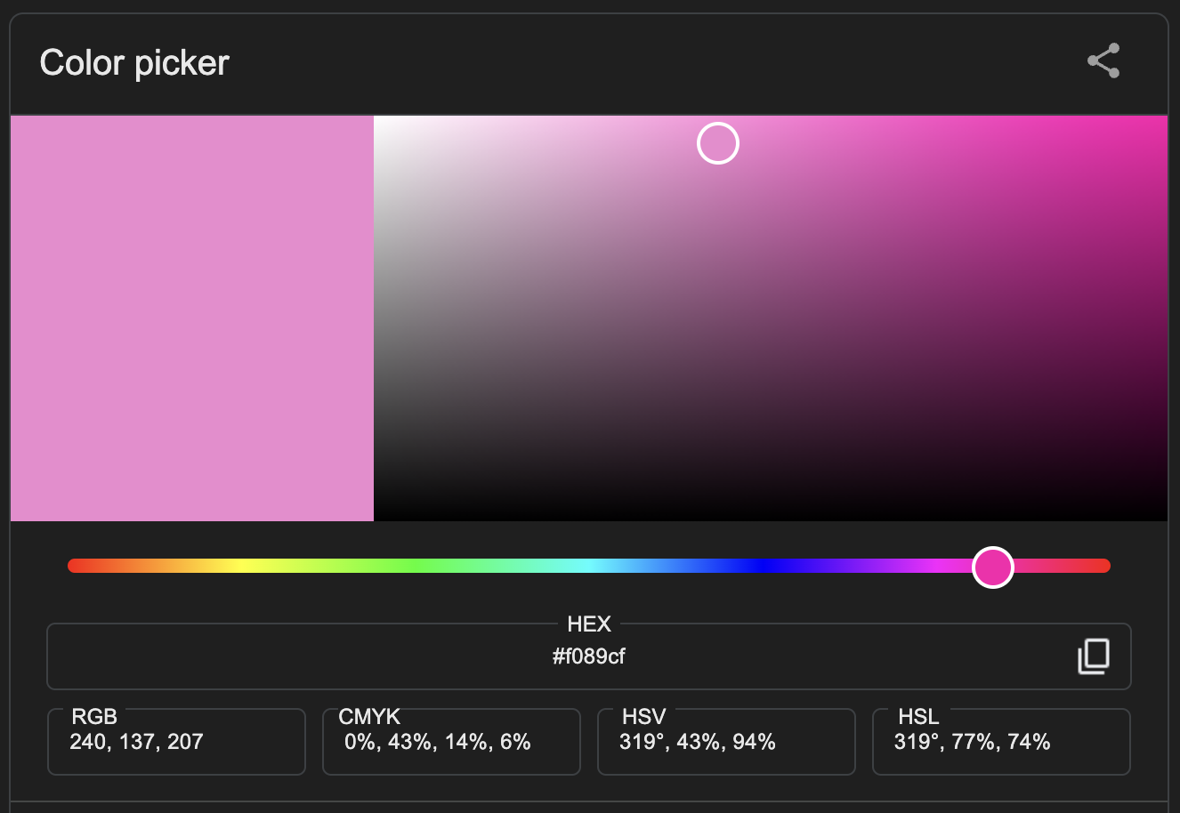
It’s probably obvious that the individual values are 137, 207 and 240, but consider that the binary representation of this color looks like this:

[ 1, 0, 0, 0, 1, 0, 0, 1, 1, 1, 0, 0, 1, 1, 1, 1, 1, 1, 1, 1, 0, 0, 0, 0 ]

And that’s just a single pixel! We talked before about how the byte array of pixels is just a flat blob of bits. Take a high definition photo, it might be 1920 x 1080 pixels or ~2.1 million pixels. Think about that compared to the single pixel array up above, because that’s a lot of data without an obvious place to start or stop! It’s easy to see how getting off by 1 or 2 bits could really change the outcome of our image.

Fortunately, PNGs provide us with everything we need to pull pixels out of this haystack of 0s and 1s. To derive the number of bits in a single pixel, we combine bitDepth and colorType. There are 5 different color types, but for the purposes of this blog post, we’ll be focusing on grayscale. (Read more about different color types and their associated bit depths in the spec.)

A Color Type will only support certain Bit Depths. Grayscale is represented by two color type codes: 0 and 4. 0 indicates grayscale without transparency (alpha), and 4 indicates grayscale with transparency. Color type 4 supports bit depths of 8 and 16, while Color Type 0 supports all bit depths (1, 2, 4, 8, and 16).

You might be thinking, “ok, that’s interesting, but what does it mean?” Essentially, your colorType will tell you how many individual values make up a pixel, and your bitDepth will tell you how many bits make up an individual value.

So using my sample photo as an example:

let bitsPerPixel = colorChannelMatrix[colorType] * bitDepth // 1 * 8

For my image, the color type is 0, which indicates a single numerical value represents each pixel. The bit depth is 8, which indicates we need to parse 8 bits at a time to find the value for each pixel. Now we will use width to determine how many bits are in a row, and then convert that to bytes.

let bitsPerRow = bitsPerPixel * width // 8 * 150

let bytesPerRow = Math.ceil(bitsPerRow / 8) // 1200 / 8

Remember, while the sample image allocates 8 bits per pixel, or exactly one byte, it’s possible for a pixel to be larger or even smaller than a single byte. That’s why we first calculate the pixel size in bits and then convert to bytes.

Now that we know how many bytes are in a row, let’s continue:

function parsePixels(signature, pixels) {
  const { height, width, colorType, bitDepth } = signature

  // the product of the colorType and bitDepth determines the bits per pixel
  let bitsPerPixel = colorChannelMatrix[colorType] * bitDepth

  // using the derived bits per pixel * width, find the bits per row / scanline
  let bitsPerRow = bitsPerPixel * width

  // finally divide that by 8 to find the bytes per row
  let bytesPerRow = Math.ceil(bitsPerRow / 8)

+ const numScanlines = height
+ let currentScanline = 0
+ const scanlineLength = bytesPerRow + 1 // add one for the filterByte

  // a matrix containing pixel values per row
+ const pixelMap = []

+ while (currentScanline < numScanlines) { /* ... */}
}

This sets us up to loop over the pixels buffer array, knowing where a given row of pixels ends, and how many totals rows to expect. scanlineLength is the number of bytes per row plus one. This is because the first pixel of a row is allocated for the filter type. This was my favorite part of PNGs! I think filter types are so clever, and deserve their own post, so we’ll cover them next.

Let’s continue on the loop:

function parsePixels(signature, pixels) {
  const { height, width, colorType, bitDepth } = signature

  // the product of the colorType and bitDepth determines the bits per pixel
  let bitsPerPixel = colorChannelMatrix[colorType] * bitDepth

  // using the derived bits per pixel * width, find the bits per row / scanline
  let bitsPerRow = bitsPerPixel * width

  // finally divide that by 8 to find the bytes per row
  let bytesPerRow = Math.ceil(bitsPerRow / 8)

  const numScanlines = height
  let currentScanline = 0
  const scanlineLength = bytesPerRow + 1 // add one for the filterByte

  // a matrix containing pixel values per row
  const pixelMap = []

  while (currentScanline < numScanlines) {
    // keep reference to initial offset
+   let startingOffset = currentScanline

    // increment row offset
+   currentScanline++

    // slice the scanline to get the current row's values
+   let row = pixels.subarray(startingOffset, startingOffset + scanlineLength)
+   let filteredRow = []

    // find the filter type and set the offset
+   let filterType = row[0];

    // set the offset to 1 to skip the filter type value
+   let offset = 1;

    // loop over the row itself
+   while (offset < row.length) {
+     let i = offset;

      // log out the current pixel value
+     console.log(row[i])

+     offset++;
+   }

    return {
      signature,
      pixelMap,
    }
  }
}

Let’s recap. At the beginning of this post we had a flat byte array and the PNG’s signature. We used the signature to derive the number of bits per pixel, and how many individual numbers make up the pixel. We also determined how many pixels are in a row, and how many rows make up the image. With all of this information, we’re now looping over the image accessing individual pixel values - wow!

Are we done? If we take these pixel values and dump them into another file, will we be duplicating the PNG? Maybe, but probably not. There’s one more step, and that’s to apply the filter type. I’ll cover that in the next post.

We left off the last post having successfully parsed the IHDR chunk, revealing metadata about the image.

Here’s the image I’m working against:

And here’s the final output of this post.

The IHDR chunk fully parsed provides this information:

{
  "width": 150,
  "height": 200,
  "bitDepth": 8,
  "colorType": 0,
  "compression": 0,
  "filter": 0,
  "interlace": 0
}

Now that we have the image metadata, let’s parse the rest of the image!

We’ll start by adding to our loop:

function parsePng(data) {
  let width;
  let height;
  let bitDepth;
  let colorType;
  let compression;
  let filter;
  let interlace;

  // this will hold the pixel bytes as we pull them from the image
+ let idatBuffers = []

  // first handle for the signature
  let i = 8;
+ let futureBufLength = 0

  // loop over the data
  while (i < data.length) {
    // find the length of the current chunk
    let chunkLength = data.readUInt32BE(i);

    // find the type of the current chunk
    let chunkName = data.toString("ascii", i + 4, i + 8);

+   let chunkData = data.subarray(i + 8, i + 8 + chunkLength)

    // access IHDR
    if (chunkName == "IHDR") {
      // create an offset to set the position at the beginning of the data section
      let ihdr = i + 8;

      // parse the header data
      width = data.readUInt32BE(ihdr);
      height = data.readUInt32BE(ihdr + 4);
      bitDepth = data[ihdr + 8];
      colorType = data[ihdr + 9];
      compression = data[ihdr + 10];
      filter = data[ihdr + 11];
      interlace = data[ihdr + 12];
    }

    // get each chunk of pixels
+   if (chunkName == 'IDAT') {
+     idatBuffers.push(chunkData)
+     futureBufLength += chunkLength
+   }

    // update the offset
    i = i + chunkLength + 12;
  }

  // return the header data
  return {
    width,
    height,
    bitDepth,
    colorType,
    compression,
    filter,
    interlace,
  };
}

In the last post, we talked about how there are no spaces between chunks, so updating the offset will bring us to the beginning of the next chunk. For us, the next chunk we care about is the IDAT chunk.

There can be multiple image data (IDAT) chunks, and these chunks take on the structure of any other chunk. Their first four bytes will contain the length of the data section. The next four will indicate the chunk type. After the type, we’re finally accessing the actual data, phew!

Within our IDAT if-block, it’s pretty straightforward. We use chunkData, which is a Buffer array containing only the data, and we push that into idatBuffers which will be our reference to our pixels.

Now that we have our pixels in an array, we’re ready for the next step.

const zlib = require('zlib')

function parsePng(data) {
  let width
  let height
  let bitDepth
  let colorType
  let compression
  let filter
  let interlace

  // this will hold the pixel bytes as we pull them from the image
  let idatBuffers = []

  // loop over the data
  // first handle for the signature
  let i = 8
  let futureBufLength = 0

  while (i < data.length) {
    let chunkLength = data.readUInt32BE(i)
    let chunkName = data.toString('ascii', i + 4, i + 8)
    let chunkData = data.subarray(i + 8, i + 8 + chunkLength)

    // get and set the signature
    if (chunkName == 'IHDR') {
      let ihdr = i + 8
      width = data.readUInt32BE(ihdr)
      height = data.readUInt32BE(ihdr + 4)
      bitDepth = data[ihdr + 8]
      colorType = data[ihdr + 9]
      compression = data[ihdr + 10]
      filter = data[ihdr + 11]
      interlace = data[ihdr + 12]
    }

    // get each chunk of pixels
    if (chunkName == 'IDAT') {
      idatBuffers.push(chunkData)
      futureBufLength += chunkLength
    }

    // signifies the end of the file
    // since we are all the way through the file, return the signature and pixels
+   if (chunkName == 'IEND') {
+     const pixel = Buffer.concat(idatBuffers, futureBufLength)

+     try {
+       let decompressed = zlib.inflateSync(pixel)

+       return {
+         signature: {
+           width,
+           height,
+           bitDepth,
+           colorType,
+           compression,
+           filter,
+           interlace,
+         },
+         pixelBytes: decompressed,
+       }
+     } catch (err) {
+       console.error('Failed to decompress:', err)
+       return
+     }
    }

    i = i + chunkLength + 12
  }
}

The last chunk of a valid PNG will always be the IEND chunk. Its data section will be empty, so once we find this chunk, we know we’re at the end of our file stream.

A few things happen here:

First, we create a new Buffer array with all of our pixel bytes (note that even though the idatBuffer array was a nested array, the pixel array will be flat).

That’s not the important part though - the most important part of this new set of code is here: zlib.inflateSync(pixel). PNGs compress their pixel data using zlib compression. You can find more information about this here in the spec.

We’re using the Node zlib library to “inflate” or decompress the pixel data. I plan to manually implement the algorithm in the future, but for now, we’ll just use the library.

Now that we have the image metadata (signature) and the raw pixels – we’re ready to get started! Check out the next blog post where we finally start decoding these pixels!

This blog post is the first in a series about image manipulation and parsing. This project started because I was curious how I might go about manually resizing an image. I’m also experimenting with manual image generation as a part of this project.

If you’d like to follow along as we go, the repo for the project is here. The PNG spec is here.

Here is the image I used:

libpng also has a comprehensive suite of images to use in tests.

Let’s jump in.

The question: What do the internals of an image actually look like?

It started with curiosity around this question: “What actually is an image? What does it look like under the hood?” Obviously different image formats will look different interally, so I had to pick one to start with, and I chose PNGs. Why PNGs? I didn’t have any particular reasoning behind selecting PNGs as my test case. Since I work on a Mac, I thought being able to generate my own PNG samples via screenshots might make this easier. That turned out not to be the case, but more on that later.

I knew there was only one to find out – crack open the file and look inside.

PNG Internals

While there are many different chunk types defined for a PNG, only three are absolutely required for a valid PNG. The IHDR chunk, at least one IDAT chunk (although there could be multiple, depending on the size of the image), and lastly the IEND chunk.

Because the goal of my project was not to write a brand new PNG viewer (although, that could happen in a future post!), I focused only on the absolutely necessary parts. As such, this post will not cover chunk types outside of IHDR, IDAT, and IEND.

Note: If you’d like to learn more, all chunk types are covered in the spec.

IHDR Values and Structure

PNGs are made up of multiple different “chunks”. In order to be a valid PNG, the first chunk must be the IHDR chunk. The Image Header chunk (IHDR) contains, you guessed it, information about the image. It is always 13 bytes and contains the following information, which will always be in this order:

• Width (in pixels)
• Height (in pixels)
• Bit depth
• Color type
• Compression method
• Filter method
• Interlace method

I’ll explain more about these in the next post. For now, just know that since the image is a flat array of bytes, we need all of this information to derive information such as: where a row of pixels starts and stops, how many bits or bytes make up a single pixel, how many color channels are used, and more. For now, we’ll focus on parsing out this information.

Parsing the IHDR

Here is an example from my project to parse the IHDR chunk.

First, we need to handle for the PNG signature. The signature is always 8 bytes (bytes, not bits), and contains the same decimal values. These values indicate the file type is a PNG. Since we know we’re parsing a PNG, we’ll just skip the signature.

Our method will take the buffer response from reading the file as it’s parameter.

function parsePng(data) {
  // the variables we are looking for from the IHDR chunk
  let width;
  let height;
  let bitDepth;
  let colorType;
  let compression;
  let filter;
  let interlace;

  // first handle for the signature
  let i = 8;
}

So far, it’s pretty straightforward. The data parameter is a buffer (an array of bytes). After we instantiate the variables we plan to parse out of IHDR, we create our offset, which skips the first 8 bytes. Next we would start looping over the buffer, but before we get too far into that, let’s talk about chunk structure.

In the first section, I mentioned that the PNG buffer is a flat array of bytes - that means there are no delimiters to signal the end of a line or the beginning of the next line. There’s also no delimiter between chunks. In fact, there are no spaces or empty bytes at all between any of the sections of a PNG. However, it’s possible to derive when you’re at the end of a chunk, based on the structure.

A chunk is made up of four parts:

• Length - the first 4 bytes of a chunk indicate the length of the data section. It’s important to note that this length is not the length of the current chunk. It is only representative of the data within the chunk.
• Type - the next 4 bytes tell you the type (name) of the current chunk
• Data - this is the part we are really after! This is the only part of a chunk with a dynamic length. All other sections are 4 bytes long.
• CRC - the final 4 bytes of a chunk. It’s essentially a checksum to validate your offsets

Every single chunk type will follow this structure and order, including IHDR and IDAT chunks.

Now that we know a little more about what we’re looking at, let’s continue:

function parsePng(data) {
  let width;
  let height;
  let bitDepth;
  let colorType;
  let compression;
  let filter;
  let interlace;

  // first handle for the signature
  let i = 8;

  // loop over the data
+  while (i < data.length) {
    // find the length of the current chunk
+    let chunkDataLength = data.readUInt32BE(i);

    // update the offset
+    i = i + chunkLength + 12;
+  }
}

We’ve added the loop and the first building blocks we need. In the loop, we first find the length of the data section, and then we use that to update the loop’s offset. We take the current position in the buffer, and add the data length (because this is the part of a chunk whose length is dynamic) + 12 bytes, to cover the rest of the chunk. Remember, there are no spaces or empty bytes between chunks, so this offset will take us to the very first byte of the following chunk.

Now we’re ready to parse the IHDR chunk:

function parsePng(data) {
  let width;
  let height;
  let bitDepth;
  let colorType;
  let compression;
  let filter;
  let interlace;

  // first handle for the signature
  let i = 8;

  // loop over the data
  while (i < data.length) {
    // find the length of the current chunk
    let chunkLength = data.readUInt32BE(i);

    // find the type of the current chunk
+   let chunkName = data.toString("ascii", i + 4, i + 8);

    // access IHDR
+   if (chunkName == "IHDR") {
      // create an offset to set the position at the beginning of the data section
+     let ihdr = i + 8;

      // parse the header data
+     width = data.readUInt32BE(ihdr);
+     height = data.readUInt32BE(ihdr + 4);
+     bitDepth = data[ihdr + 8];
+     colorType = data[ihdr + 9];
+     compression = data[ihdr + 10];
+     filter = data[ihdr + 11];
+     interlace = data[ihdr + 12];
+   }

    // update the offset
    i = i + chunkLength + 12;
  }

  // return the header data
+ return {
+   width,
+   height,
+   bitDepth,
+   colorType,
+   compression,
+   filter,
+   interlace,
+ };
}

You might notice a difference between the way we treat the first value within a chunk (length) and the next value (type). The length is always 32-bit integer, whereas the chunk type is always 4 ASCII characters. Because these are different data types, we must access their values differently.

The next bit of code is very straightforward. We identify the IHDR chunk and set the header values. Notice again that the first two values are treated differently than the next five. Because those first two initial values are 32-bit integers, we need to parse all four bytes together to find the correct value for each.

The final five values are all single byte values, so they can be directly accessed.

The image header for the test image I used looked like this:

{
  "width": 150,
  "height": 200,
  "bitDepth": 8,
  "colorType": 0,
  "compression": 0,
  "filter": 0,
  "interlace": 0
}

Now that we have the image header information, we’re ready to get into the actual pixel values of the PNG! I’ll cover that in the next blog post.

Lately I’ve been doing a lot more data-driven work, including data analysis. From this work, I’ve needed to import and export a lot of data. Here is my best quick-and-dirty way to copy a table from one Postgres table to another. I frequently use this method to refresh my local environment with production data.

Of course, if you’re using a tool like pgAdmin, you can export data at the click of a button, but depending on what you plan to do with the data, that may not be what you want to do. Using the pgAdmin export will include all of the record IDs, so if you’re using this data to augment another database (or in my case, refresh), this might not be what you want. But if that doesn’t matter, using a built-in import/export tool is definitely the easiest solution.

Unfortunately this usually doesn’t work for me, so this is what I do instead:

Export the prod data into a CSV

\copy (select columnA, columnB, columnC from tablename) to 'absolute/path/plus/file.csv' csv DELIMITER ',';

Make sure you include the absolute filepath, otherwise you’ll have a lot of trouble finding your csv. (This is the absolute path to your local machine.)

You can include any query above, so if you need to filter or sort in a certain way, adjust your query accordingly.

Drop the data from my local database and reset the sequence

Make triple-sure you’re in the correct environment before you do this!!

truncate tablename;

select nextval('sequencenameforprimarykey');
alter sequence sequencename restart with 1;

select nextval('sequencenameforprimarykey');
select count(*) from tablename

After you truncate your table and reset your sequence, you can select each and see that you’re ready to start fresh with your prod data.

Insert data from the CSV

\copy table_name(columnA, columnB, columnC) from 'absolute/path/plus/file.csv' csv DELIMITER ',';

Notice that the above command is basically just the inverse of the first \copy command in step 1.

Depending on how much data you’re copying over, this step might take a while. At the end, you’ll see something like COPY 137 in your terminal, which indicates the copy is complete and 137 records were copied into your table.

I’ll usually use one more select count(*) from tablename to see the total number of records in the table, as a sanity check.

A few gotchas to watch for:

Permission denied errors

If you used \COPY without root permissions, try again with \copy. The \COPY command has a slightly different signature and requires root access, but \copy will work regardless.

“Cannot insert {type} into column”

An issue of incorrect data to column type. When this happens to me, it usually means I forgot to specify the columns in my \copy to command, or I specified them in the wrong order. If you are going to ignore the IDs when you move data from one place to another – which is a good idea – you must specify the columns in your \copy to command!

“Missing data for column”

When this happens to me, it usually means I forgot to specify the delimiter to be a comma in my \copy to command. Check your CSV file and ensure that you’re using the correct delimiter for your data.

“Duplicate key value violates unique constraint”

Most likely cause is that you copied your entire table, including ids, but forgot to drop your secondary table’s data and/or reset the sequence.

And that’s about it! At this point, I’ve copied production data into a local or sandbox environment where its safe to tinker with or even delete data. Just be careful and always, always, always make sure you’re not in production when tinkering!

Happy SQL-ing!